It is more likely that a good model will learn to choose a small parameter value, like 0.1, when a possible range of values of a feature is large, like 2000.
In other words, when the possible values of the feature are small, then a reasonable value for its parameters will be large.
prediction price = w1*x1 + w2*x2 + b
x1 : size –> range 300 – 2000 ==> large
x2 : # of bedrooms –> range 0 – 5 ==> small
x1 = 2000 , x2 = 5, price = 500K w1 and w2?
if w1 = 50, w2 = 0.1, b= 50 ==> 100,050.5K ==> very far from the actual price
if w1 = 0.1, w2 = 50, b=50 ==> 500K ==> same price
small change to w1 can have a very large impact on the cost and estimated price.
solution : to scale the features x1 and x2 (between 0 and 1)
If you run gradient descent on a cost function to find w and b on this rescaled x1 and x2, then it will be faster.
When you have different features that take on very different range of values, it can cause gradient descent to run slowly.
BUT rescaling the different features, so they all take on comparable/similar range of values and speed up gradient descent significantly.
rescale => to take features that take on very different range of values and skill them to have comparable ranges of values to each other.
1 – dividing by maximum
300 <= x1 <= 2000, 0<= x2 <= 5
x1_scaled = x1/2000, x2_scaled = x2/5
0.15 <= x1_scaled <= 1, 0 <= x2_scaled <= 1
2 – mean normalization : find the average
lets say avr_x1 = 600, avr_x2 = 2.3
(x1 – 600) / (2000 – 300) ==> (300 – 600) / 1700, (2000-600) / 1700 ==> -0.18<= x1_scaled <= 0.82
(x2-2.3) / (5 – 0) ==> (0-2.3) / 5 , (5-2.3) / 5 ==> -0.46 <= x2_scaled <= 0.54
3- z-score normalization
(x1 – average) / standard deviation
Acceptable ranges
-1 <= x_j <= 1
-3 <= x_j <= 3
-0.3 <= x_j <= 0.3
0 <= x_j <= 3
-2<= x_j <= 0.5
Need to rescale
-100 <= x_j <= 100. ==> too large
-0.001 <= x_j <= 0.001 ==> too small
98.6 <= x_j <= 105 ==> too large
As below code shows:
by using normalization and when number of iteration is 100 and alpha is 0.0000001,
cost is 1576.084
by using normalization and when number of iteration is 100 and alpha is 0.1,
cost 221.22
import matplotlib.pyplot as plt
import numpy as np
import matplotlib.pyplot as plt
def load_house_data():
data = np.loadtxt("/Users/ozgeguney/PycharmProjects/pythonProject/data/houses.txt", delimiter=',', skiprows=1)
X = data[:,:4]
y = data[:,4]
return X, y
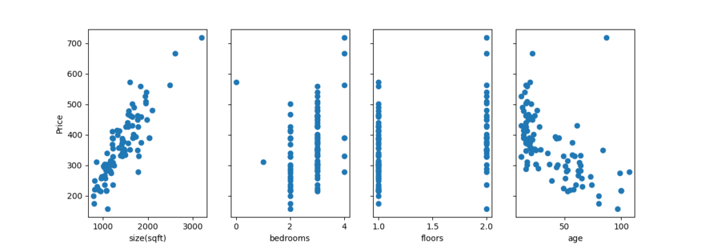
X_train, y_train = load_house_data()
X_features = ['size(sqft)','bedrooms','floors','age']
fig,ax = plt.subplots(1,4, figsize=(12,3), sharey=True)
for i in range(len(ax)):
ax[i].scatter(X_train[:,i], y_train)
ax[i].set_xlabel(X_features[i])
ax[0].set_ylabel("Price")
#plt.show()
def compute_cost(X, y, w, b):
m = X.shape[0]
cost =0
for i in range(m):
fx= np.dot(X[i],w) + b
cost += (fx-y[i])**2
cost = cost/(2*m) #np.squeeze(cost)
print(cost)
return cost
def compute_cost_matrix(X, y, w, b):
fx = X @ w + b
err = np.sum((fx - y)**2)/(2*X.shape[0])
print(err)
return err
def compute_gradient(X,y,w,b):
m,n = X.shape
djw = np.zeros(n)
djb = 0
for i in range(m):
fx = np.dot(X[i],w) + b
err = fx - y[i]
for j in range(n):
djw[j] += err * X[i,j]
djb += err
djw = djw / m
djb = djb / m
return djw, djb
def compute_gradient_matrix(X, y, w, b):
m = X.shape[0]
# calculate fx for all examples.
fx = X @ w + b # x: m,n w: n, fx: m
err = fx - y
djw = (X.T @ err)/m
djb = np.sum(err)/ m
return djw,djb
def run_gradient_descent(x,y,iteration,alpha):
w_initial = np.zeros(x.shape[1])
b_initial =0
w_out, b_out = gradient_descent_houses(x,y,w_initial,b_initial, alpha, iteration, compute_gradient )
#print(f"w,b found by gradient descent: w: {w_out}, b: {b_out:0.2f}")
print(w_out,b_out)
return (w_out, b_out)
import copy
def gradient_descent_houses(X,y,w,b,alpha,iteration,gradient_function):
m = len(X)
w_temp = copy.deepcopy(w)
b_temp = b
for i in range(iteration):
djw,djb =gradient_function(X,y,w_temp,b_temp)
w_temp = w_temp - alpha*djw
b_temp = b_temp - alpha*djb
return w_temp, b_temp
w_out, b_out= run_gradient_descent(X_train,y_train,100,0.0000001)
compute_cost(X_train,y_train,w_out,b_out)
compute_cost_matrix(X_train,y_train,w_out,b_out)
def zscore_normalize_features(X):
mu = np.mean(X, axis=0)
sigma = np.std(X, axis=0)
X_norm = (X - mu) / sigma
return (X_norm)
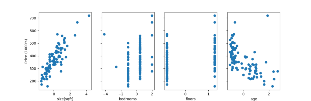
X_norm= zscore_normalize_features(X_train)
fig,ax=plt.subplots(1, 4, figsize=(12, 3), sharey=True)
for i in range(len(ax)):
ax[i].scatter(X_norm[:,i],y_train)
ax[i].set_xlabel(X_features[i])
ax[0].set_ylabel("Price (1000's)")
#plt.show()
#The scaled features get very accurate results much, much faster!
#Notice the gradient of each parameter is tiny by the end of this fairly short run.
w_out, b_out= run_gradient_descent(X_norm,y_train,100,0.1)
compute_cost(X_norm,y_train,w_out,b_out)data address : https://github.com/ozgeguney/Machine-Learning/blob/main/houses.txt
Thank you Andrew Ng, thank you Coursera:)
Reference: https://www.coursera.org/learn/machine-learning/home/week/2
then, let’s continue with Feature Engineering