How can linear regression model complex, even highly non-linear functions using feature engineering?
The choice of features can have a huge impact on your learning algorithm’s performance
Feature engineering : using domain knowledge to design new features, by transforming a feature or combining original features
f(x) = w1*x1 + w2*b2 + b
x1 : frontage
x2: depth
area = frontage * depth
x3 = x1*x2 (new feature)
f(x) = w1*x1 + w2*x2 + w3*x3 + b
the model can now choose parameters w_1, w_2, and w_3, depending on whether the data that the frontage or the depth or the area x_3 shows the most important thing for predicting the price of the house.
polynomial regression
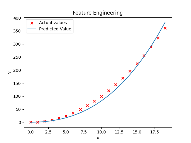
It doesn’t look like a straight line fits this data-set very well. Maybe you want to fit a curve, maybe a quadratic function to the data like this which includes a size x and also x squared. Maybe that will give you a better fit to the data.
f(x) = w1*x + w2*x**2 + w3*x**3 + b
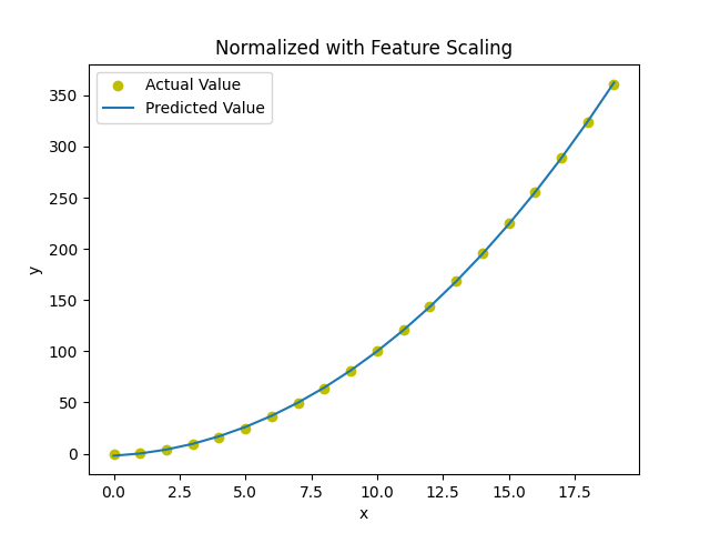
It’s important to apply feature scaling to get your features into comparable ranges of values.
as below code shows:
without normalization: w,b found by gradient descent: w: [0.08237526 0.53552137 0.02752216], b: 0.0106
with normalization: w,b found by gradient descent: w: [ 7.67449373 93.94625791 12.28868959], b: 123.5000
As can be seen from the values here, w1 is important (x^2).
import numpy as np
import matplotlib.pyplot as plt
from BasicFunctions import zscore_normalize_features, run_gradient_descent, compute_cost_matrix
x = np.arange(0,20,1)
y = x**2
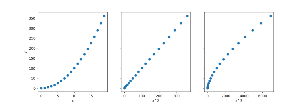
X = np.c_[x,x**2,x**3]
w, b = run_gradient_descent(X,y,10000,0.0000001)
y_predicted = X @ w + b
plt.scatter(x,y, c="r", marker="x", label="Actual values")
plt.title("Feature Engineering")
plt.plot(x, y_predicted, label = "Predicted Value")
plt.xlabel("x")
plt.ylabel("y")
plt.legend()
X_features = ["x","x^2","x^3"]
fig,ax = plt.subplots(1,3,figsize=(12,3), sharey= True)
for i in range(len(ax)):
ax[i].scatter(X[:,i],y)
ax[i].set_xlabel(X_features[i])
ax[0].set_ylabel("y")
X = zscore_normalize_features(X)
w, b = run_gradient_descent(X,y,10000,0.1)
compute_cost_matrix(X,y,w,b)
y_predicted = X @ w + b
fig1 = plt.figure("Figure 3")
plt.scatter(x, y, marker="o", c= "y",label= "Actual Value")
plt.title("Normalized with Feature Scaling")
plt.plot(x,y_predicted,label="Predicted Value")
plt.xlabel("x")
plt.ylabel("y")
plt.legend()
plt.show()