The gradient descent can be guaranteed to converge to the global minimum. If using the mean squared error for logistic regression, the cost function is non-convex. So, it is more difficult for gradient descent to find an optimal value for w and b.
Linear Regression => squared error. cost -> convex
Logistic Regression ==> if we use squared error cost function, non-convex. There are lots of local minima. not good choice to use squared error cost function.
Loss => on a single training example.
Cost => J(w,b) = by summing up the losses on all of training examples. Then, average.
Logistic Loss Function
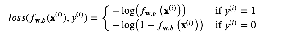
f(x) = 1 then use -log(f(x)) ==> loss 0 🙂
f(x) = 0.5 -log(0.5) = 0.3 ==> loss = 0.3 high
f(x) =0 -log(1-0) = 0 ==> loss =0
The loss function above can be rewritten to be easier to implement.

cost = J(w,b) = 1/ m (sum L(f(x)))
That is convex ==> can reach a global minimum.
f(x) = g(z) z = wx + b. g(z) = 1 / 1 + e-z
z_i = np.dot(x[i],w) + b
f_wb_i = sigmoid(z_i)
cost += (-y[i]* np.log(f_wb_i))) – (1-y[i])*log(1- f_wb_i))
cost = cost / m
Linear Regression : f(x) = wx + b
Logistic Regression : 1 / 1 + e-(wx+b)
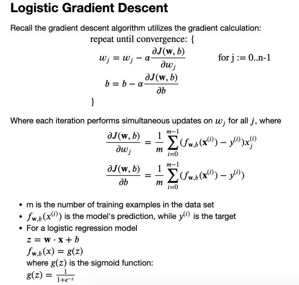
We are going to find the values of parameters w and b that minimize the cost function J(w,b). We will again apply gradient descent to do this. Find w and b.
again derivative of cost function :
log derivative: y = logX y‘ = 1/x
y = log(f(X)) y‘ = f(x)‘ /f(x)
y = ex y‘ = ex
y = ef(x) y‘ = f(x)‘ . ef(x)
SAME CONSEPT:
Monitor gradient descent
Vectorized implementation
Feature Scaling: to take on similar range of values -1<x[i]<1
Vectorized implementation and Feature Scaling ==> gradient descent faster
import numpy as np
import matplotlib.pyplot as plt
X_train = np.array([[0.5, 1.5], [1,1], [1.5, 0.5], [3, 0.5], [2, 2], [1, 2.5]]) #(m,n)
y_train = np.array([0, 0, 0, 1, 1, 1]) #(m,)
def plot_data(X, y, ax, pos_label="y=1", neg_label="y=0", s=80, loc='best' ):
pos = y == 1
neg = y == 0
pos = pos.reshape(-1,) #work with 1D or 1D y vectors
neg = neg.reshape(-1,)
# Plot examples
ax.scatter(X[pos, 0], X[pos, 1], marker='x', s=s, c = 'red', label=pos_label)
ax.scatter(X[neg, 0], X[neg, 1], marker='o', s=s, label=neg_label, c="blue", lw=3)
ax.legend(loc=loc)
ax.figure.canvas.toolbar_visible = False
ax.figure.canvas.header_visible = False
ax.figure.canvas.footer_visible = False
fig,ax = plt.subplots(1,1,figsize=(4,4))
plot_data(X_train, y_train, ax)
# Set both axes to be from 0-4
ax.axis([0, 4, 0, 3.5])
ax.set_ylabel('$x_1$', fontsize=12)
ax.set_xlabel('$x_0$', fontsize=12)
plt.show()
def compute_cost_function(X,y,w,b):
m = X.shape[0]
cost =0.0
for i in range(m):
z_i = np.dot(X[i],w) + b
f_wb_i = 1 / (1 + np.exp(-z_i))
cost += -y[i]*np.log(f_wb_i) - (1-y[i])*np.log(1-f_wb_i)
cost = cost / m
return cost
w = np.array([1,1])
b = -3
print(compute_cost_function(X_train, y_train, w, b))
# Choose values between 0 and 6
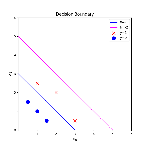
x0 = np.arange(0,6)
# Plot the two decision boundaries
x1 = 3 - x0
x1_other = 5 - x0
fig,ax = plt.subplots(1, 1, figsize=(6,6))
# Plot the decision boundary
ax.plot(x0,x1, c="blue", label="$b$=-3")
ax.plot(x0,x1_other, c="magenta", label="$b$=-5")
# Plot the original data
plot_data(X_train,y_train,ax)
ax.axis([0, 6, 0, 6])
ax.set_ylabel('$x_1$', fontsize=12)
ax.set_xlabel('$x_0$', fontsize=12)
plt.legend(loc="upper right")
plt.title("Decision Boundary")
plt.show()decision boundary => z = wx+b =0
continue to the problem of overfitting