for binary classification problems
y can only be one of two values/two classes/two categories.
yes or no
true or false
1 or 0

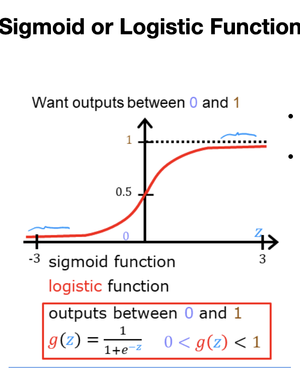
Logistic Regression is a fit curve that looks like S shape curve to the dataset.
it uses sigmoid function. Sigmoid function outputs value is between 0 and 1.

g(z) = 1 / (1 + e^-z). 0 < g(z)<1
if z =100 e^-z ==> very tiny number g(z) ~ 1
if z large g(z) ~ 1
if z=-100 e^-z ==>2.7^100 g(z) ~ 0
if z large negative g(z) ~ 0
if z=0 e^-0=1 g(z) = 1 / (1+1) = 0.5
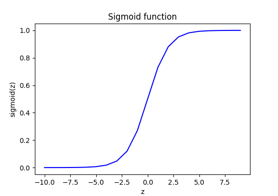
the sigmoid function approaches 0 as z goes to large negative values and approaches 1 as z goes to large positive values.

import numpy as np
import matplotlib.pyplot as plt

def sigmoid(z):
    g = 1 / (1 + np.exp(-z))
    return g

z_temp = np.arange(-10,10)
y = sigmoid(z_temp)

fig, ax = plt.subplots(1,1,figsize=(6,3))
ax.plot(z_temp, y, c="b")
ax.set_title("Sigmoid function")
ax.set_xlabel("z")
ax.set_ylabel("sigmoid(z)")
plt.show()
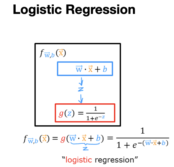
z = wx+b
f(x) = z = wx + b ==> linear regression
f(x) = g(z) = 1 / (1 + e^-(wx+b)) ==> logistic regression
output of logistic regression is probability that class “1”
f(x) = 0.7 ==> %70 chance that y is 1, %30 chance that y is 0
P(y=1| x;w,b) = f_wb(x)= g(wx+b)
pick a threshold: 0.5
if f_wb(x) >= 0.5 then y^= 1 (Yes)
else y^=0 (No)
f_wb(x) >= 0.5
g(z)=>0.5
z>=0
wx+b>=0 then y^=1
wx+b<0 then y^=0
decision boundary => z = wx+b =0
non-linear decision boundary : z = x1^2 + x2^2 -1 =0 x1^2 + x2^2 = 1
x1^2 + x2^2 >= 1 y^ = 1
x1^2 + x2^2 < 1 y^ = 0
you should use a low threshold, you don’t want to miss.