Gradient Descent

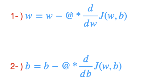
Gradient Descent finds better and better values for the parameters w and b. It uses below equation.
@ : learning rate controls how big step you take. It is a small number between 0 and 1. It might be 0.01.
Derivative term : in which direction you want to take your baby step
Derivative term in combination with the learning rate @, it determines the size and direction of step you want to take downhill.

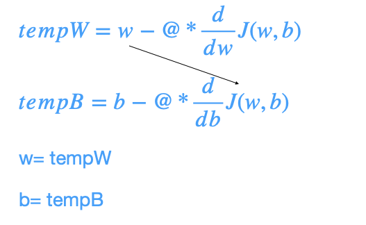
Repeat 1st and 2nd step until convergence
By converges, the parameters w and b no longer change much with additional step and you reach the point at a local minimum. Here, it is important to update w and b simultaneously.

if @ is too small, you need a lot of steps to get to the minimum. It will be slow. It will take a very long time.
if @ is too large, you take huge step, and overshoot the minimum. In other words, you never reach minimum point. It will fail to converge and it will diverge.
if the derivative of the cost function equals zero, so slope is zero, w will not change anymore.
near a local minimum, derivatives becomes smaller.

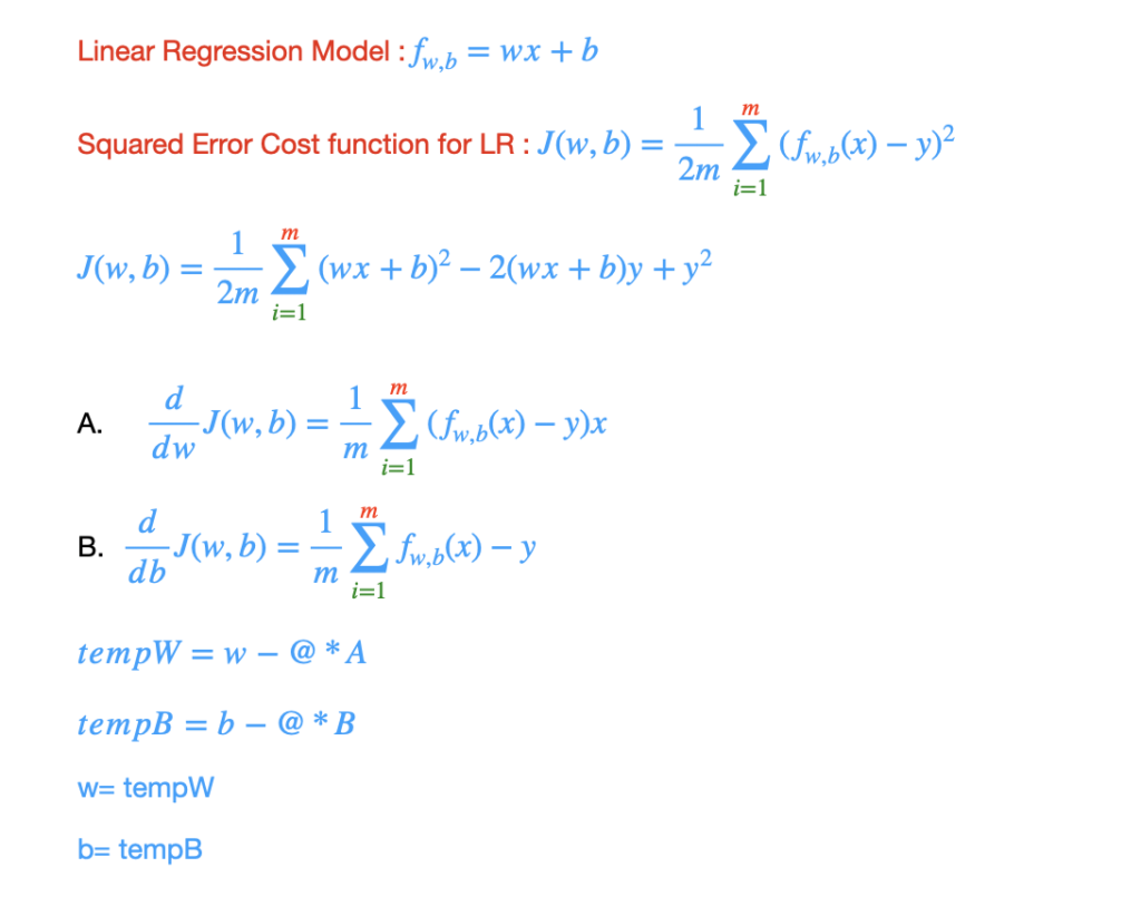
Gradient Descent for Linear Regression

It uses squared error cost function.
It is convex function.
It has a single global minimum. What is global minimum?
The point has the lowest possible value for the cost function J of all possible points.
Remember ! depending on where you initialize the parameters w and b, you can end up at different local minima. But LR cost function cannot have any local minima. It has bowl shape.

import numpy as np

x_train =np.array([1.0,2.0])
y_train =np.array([300.0, 500.0])

def compute_gradient(x, y, w, b):
    m = x.shape[0]
    dCost_w = 0
    dCost_b = 0
    for i in range(m):
        prediction = w* x[i] + b
        dCost_w += (prediction - y[i]) * x[i]
        dCost_b += prediction - y[i]
    dCost_w = dCost_w / m
    dCost_b = dCost_b / m
    return dCost_w, dCost_b

def gradient_descent(x,y, w_initial, b_initial, alpha, num_iters, gradient_function):
    w = w_initial
    b = b_initial

    w_b_history =[]
    for i in range(num_iters):
        dCost_w, dCost_b = gradient_function(x,y,w,b)
        w = w - alpha * dCost_w
        b = b - alpha * dCost_b

        w_b_history.append([w,b])

    return w,b, w_b_history

w_init = 0
b_init = 0
alpha = 0.5
iterations = 400

w_final, b_final, w_b_history = gradient_descent(x_train,y_train,w_init,b_init,alpha,iterations, compute_gradient)
print(f"(w,b) found by gradient descent: ({w_final:0.4f},{b_final:0.4f})")
print(w_b_history)

We automated the process of optimizing w and b using gradient descent.
(w,b) found by gradient descent: (200.0000,100.0000).

Batch Gradient Descent

Each step of gradient descent uses ALL training examples.
For LR, use Batch Gradient Descent

Here, the LR model has one feature, it is univariate linear regression.

If we want to handle multiple input features, use vectorization, but first look to vectors and matrices to learn how to use vectorization.